AI Time Series Forecasting with TabPFN (Python Tutorial)

Transformers work for tabular data too

This tutorial shows you how to do time series forecasting in Python of cyclical data using TabPFN, a cutting-edge transformer-based neural network. You'll see how TabPFN's "zero-shot" capabilities, achieved through extensive pre-training on synthetic datasets, allow for accurate predictions without traditional model training or hyperparameter tuning.

The video shows you how to predict U.S. housing starts from the Federal Reserve Economic Data (FRED), demonstrating how TabPFN handles cyclical and seasonal patterns effectively. You'll learn how to quickly retrieve and preprocess economic data, generate point forecasts with built-in calibrated prediction intervals, and compare results to a straightforward XGBoost benchmark for context.

Importantly, this approach excels in modeling cyclical data, such as seasonal sales, employment rates, or other business or economic data series, though it isn't suitable for strongly trending series like stock prices without additional trend modeling. This tutorial is ideal for data scientists, machine learning engineers, and analysts interested in rapid, hardware-light forecasting solutions that can be easily adapted to other cyclical data.

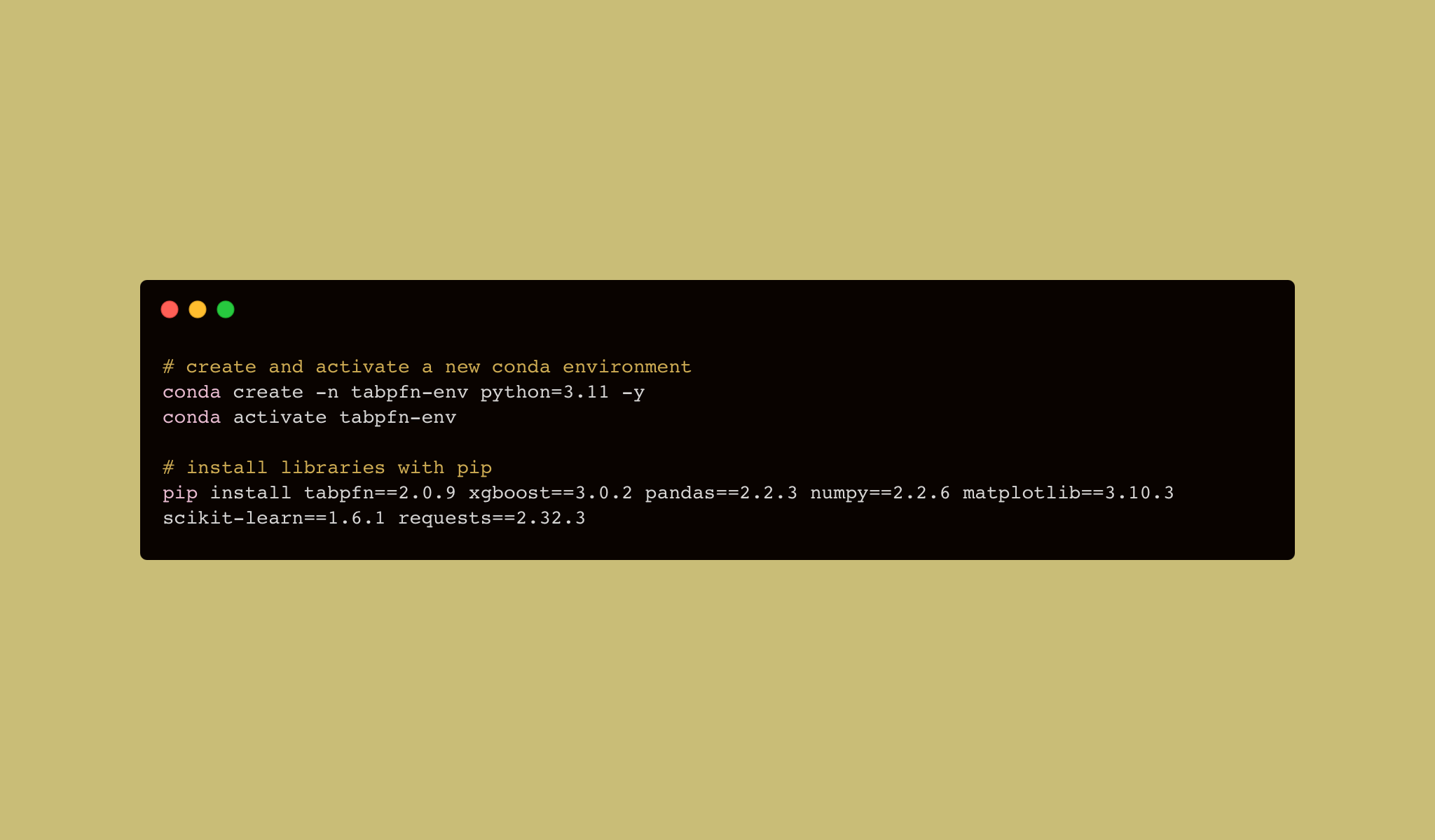
Environment Setup

Code

# Libraries
import os, io, time, requests
import pandas as pd, numpy as np, matplotlib.pyplot as plt
from tabpfn import TabPFNRegressor
from xgboost import XGBRegressor
from sklearn.metrics import mean_absolute_error

# Configurations
os.environ["TABPFN_ALLOW_CPU_LARGE_DATASET"] = "1"      # lift 1-k-row cap


# (1) Data Import
CSV_URL = "https://fred.stlouisfed.org/graph/fredgraph.csv?id=HOUSTNSA"
raw_csv = requests.get(CSV_URL, timeout=15).text       

df = (
    pd.read_csv(io.StringIO(raw_csv), parse_dates=["observation_date"])
      .rename(columns={"observation_date": "Date", "HOUSTNSA": "Value"})
      .set_index("Date")
      .sort_index()
)

# (2) Data Subset + Feature Engineering
df = df.loc["2022-01-01":]   

df["month"]   = df.index.month
df["run_idx"] = np.arange(len(df)) / len(df)


# (3) Train/Test Split
HORIZON     = 16
train, test = df.iloc[:-HORIZON], df.iloc[-HORIZON:]
X_tr, y_tr  = train.drop(columns="Value"), train["Value"]
X_te, y_te  = test.drop(columns="Value"),  test["Value"]

# (4) Model Creation

## TabPFN
tab = TabPFNRegressor(device="cpu", ignore_pretraining_limits=True)
tab.fit(X_tr.values, y_tr.values)
y_tab = tab.predict(X_te.values, output_type="median")
q10, q90 = tab.predict(X_te.values, output_type="quantiles",
                       quantiles=[0.1, 0.9])

## XGBoost
xgb = XGBRegressor()
xgb.fit(X_tr, y_tr)
y_xgb  = xgb.predict(X_te)

# (5) Comparison of Mean Absolute Error
print(f"TabPFN  MAE : {mean_absolute_error(y_te, y_tab):.2f}")
print(f"XGBoost MAE : {mean_absolute_error(y_te, y_xgb):.2f}")

# (6) Chart Comparison
plt.figure(figsize=(7,4))
plt.plot(df.index, df["Value"], label="History")
plt.plot(y_te.index, y_tab, "o-", label="TabPFN median")
plt.fill_between(y_te.index, q10, q90, alpha=.25, label="TabPFN 80 % PI")
plt.plot(y_te.index, y_xgb, "s--", label="XGBoost point-forecast")
plt.title("Housing Starts (HOUSTNSA) — TabPFN vs XGBoost")
plt.ylabel("Thousands of Units")
plt.legend(); plt.tight_layout(); plt.show()

Thanks for reading the Deep Charts Substack. Check out my new Google Sheets add-on that lets you do historical stock backtest simulations directly in Google Sheets: Stock Backtester for Google Sheets™

---

Subscribe to the Deep Charts YouTube Channel for more informative AI and Machine Learning Tutorials.